
Moments are set of statistical parameters used to describe a distribution. The calculations are simple, so are often used as a first quantitative insight into the data. A good understanding of data should always be the step before training any advanced ML model. It allows minimizing the time required to choose the methodology and interpret results.
In physics, moments refer to mass and inform us how the physical quantity is located or arranged. In math, moments refer to something similar — the probability distribution — a function that explains how probable are different possible outcomes of an experiment. To be able to compare different data sets we can describe them using the first four statistical moments:
1. The expected value
2. Variance
3. Skewness
4. Kurtosis
Let’s go through the details together!
The article is organized into two parts:
I. Math Refresher
II. Questions from data science interviews related to the topic
I. Math Refresher
1. The expected value
The first moment — the excepted value, known also as an expectation, mathematical expectation, mean, or average is the sum of all the values the variable can take times the probability of that value occurring. It can be intuitively understood as the arithmetic mean:
This is true when all outcomes have the same probability of occurrence (e.g. throw of a classical dice — all numbers from 1 to 6 have the same chance to be thrown). The more general equation including the probability of each event is:


For rolling a single die, when each value has a probability of occurrence of 1/6, the expected value would be:


Or:


For equally probable events, the expected value is the same as what the arithmetic mean. This is one of the most popular measures of central tendency, often called averages. The other common measures are:
- median — the middle value
- mode — the most likely value.
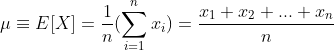
For example, taking the set of seven values: 2, 4, 4, 5, 8, 12, 14, we have:
- Mean:


- Median- this is “the middle” value, being exactly in the middle of a data set. For our example, this is 5, as it separates the greater and lesser halves of data: we have 3 values lower than five and 3 values higher than 5. For a data set with an even number of values (e.g. adding 15 to our data set), we take two values in the middle and calculate the mean out of them:

- Mode- the most frequent value in a set of data. For our example above, the mode is 4, since it appears twice.
2. Variance
The second central moment is variance. Variance explains how a set of values are spread around their expected value. For n equally likely values, the variance is:

Where μ is the average value. So the variance depends strongly on the expected value.
For the exemplar data series above, the variance is:


Where n is 7, since we have 7 elements in our data set, and μ is 7, as calculated above.
When the spread of values is lower and the same mean, the variance is also lower, e.g.:


Standard deviation
Standard deviation is a square root of the variance and is commonly used since its unit is the same as of X:


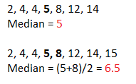
Variance and standard deviation inform us how strong data is spread around the mean, as shown in the plot below:

The greater the variance/ standard deviation (e.g. blue line), the wider the spread of values around the mean. If a variance is lower, the values are cumulated closer to the mean (red line) and the peak is higher.
The next picture summarizes the interpretation of the first two moments:


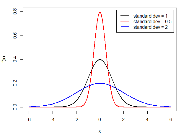
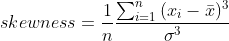
3. Skewness
Skewness, which is the third statistical moment measures asymmetry of data about its mean. The formula for calculating skewness is:
We can distinguish three types of distribution with respect to its skewness:
- symmetrical distribution: as in examples above. Both tails are symmetrical and the skewness is equal to zero.
- positive skew (right-skewed, right-tailed, skewed to the right): the right tail (with larger values) is longer. This informs us about ‘outliers’ that have values higher than the mean.
- negative skewed (left-skewed, left-tailed, skewed to the left): the left tail (with small values) is longer. This informs us about ‘outliers’ that have values lower than the mean.
In general, skewness will impact the relationship of mean, median, and mode in the following way:


- for symmetrical distribution: mean = median = mode
- for positively skewed distribution: mode < median <mean
- for negatively skewed distribution: mean < median <mode
But this is not true for all possible distributions. For example, if one tail is long, but the other is heavy, this may not work. The best way to investigate your data is to calculate all three estimators and draw conclusions based on the results, rather than general rules.
4. Kurtosis
The fourth statistical moment is kurtosis. It focuses on the tails of the distribution and explains whether the distribution is flat or rather with a high peak. Kurtosis informs us whether our distribution is richer in extreme values than normal distribution.
There is no strict consensus for the formula used to calculate kurtosis and there are three main formulas used by different programs/packages. A good habit would be to check which one is used by your software before you draw conclusions on your data. The formulas containing the correction term of minus 3 refer to the excess kurtosis. So, the excess kurtosis is equal to kurtosis minus 3.
In general, we can distinguish three types of distributions:
- Mesokurtic — having the kurtosis of 3 or excess kurtosis of 0. This group involves the normal distribution and some specific binomial distributions.
- Leptokurtic — the kurtosis is greater than 3, or excess kurtosis is greater than 0. This is the distribution with fatter tails and a more narrow peak.
- Platykurtic — the kurtosis is smaller than 3 or negative for excess kurtosis. This is a distribution with very thin tails compared to the normal distribution.
For those of you who have a better visual memory, take a look at my sketch:


We went through the first four statistical moment. It is time now for checking ourselves in the interview questions.
II. Questions from Data Science interviews
1. What is the kurtosis of normal distribution?
This is a tricky question! As mentioned in Math Refresher, there is no strict consensus for the formula used to calculate kurtosis and three formulas are commonly met. The most significant difference, especially for large samples where the choice of equation does not matter that much, is to understand whether your formula involves a correction term of -3. If so, the formula calculates excess kurtosis. This means that normal distribution may have a kurtosis of 3 or excess kurtosis of 0. But be careful since the excess kurtosis is also sometimes shortened to simpler kurtosis.
Some languages allow you to choose the type of formula in your calculations (e.g. R) or define which definition of normal kurtosis you want to use (Python). Knowing what you calculate will allow you to compare the results with normal distribution and draw conclusions.
2. When would you consider using median instead of mean?
A sample mean is a well understood and common estimator of an unknown population mean. However, it tends to be easily affected by outliers, especially when the sample size is small. So, if the data set is small, skewed, and there are outliers, it is worth checking the median.
3. You want to invest your money and have two distributions of returns available: with positive and with negative skew. Which one would you choose and why?
There is no good or bad answer here, as long as you can give a rationale for your choice. It depends on your risk appetite.
Personally, with mean and variance held constant, I would invest in positive skew. In general, having a greater chance of getting a high return costs a higher probability of having a large loss. So, in the choice between:
1. 85% chance to win at least $1000 and 1% to lose $99000 or more
2. 1% chance to win at least $99000 and 85% to lose $1000 or more
I go for the first option — a smaller but more probable win over the hope for a big win in the lottery. But the choice depends on you!
4. In your opinion, how informative is the average salary in a given country?
I believe it should be always reported together with the median. This way, we can learn much more about the salary distribution in society. For example, if there is a small group of people with super huge salaries, but the rest earns very little, it will be visible when comparing median and mean. From these two estimators, we can understand whether decent pay can be treated as normal or rather as an outlier. Of course, salaries should be alsocompared with the cost of living in a given country to get a better picture of the quality of life.
Thanks for reading!
We went together through the first four statistical moments: the expected value, variance, skewness, and kurtosis. I hope it was an exciting journey for you.
Remember that the most efficient way to learn (math) skills is by practice. So don’t wait until you feel ‘ready’, just grab a pen and paper or your favourite software and try few examples on your own. I keep my fingers crossed for you.
You may also like:
I will be happy to hear your thoughts and questions in the comments section below, reach me directly via my LinkedIn profile or at akujawska@yahoo.com. See you soon!