A Single Equation that Rules the World
The equation connects neuron firing, fluid convection, the Mandelbrot set and so much more and will definitely change your view of this world.
What if I say that the Mandelbrot set, a population of squirrels, a dripping faucet, the firing of neurons in our brain and the thermal convection is connected by one simple equation? Maybe you’ll laugh at me. But math is stranger than fiction.
Let’s dive deep into this.
Suppose you want to model a population of squirrels. This year, we have X number of squirrels. So, what might be the population next year? A simple model can be, just multiply the current population with a number. Let it be r. so, the growth rate is r. So, next year, the number of squirrels will be rX.
If r=2, it will mean that the population will double every year. But there is a problem. It implies that the population of squirrels will grow exponentially, forever. That doesn’t really happen. So, we bound it by some constrains. Let’s add the term (1-X) to the equation to represent the constraints of the environment.
So, it becomes rX(1-X). Here we are imagining X is a percentage of the theoretical maximum. X goes from 0 to 1 and as it approaches 1, (1-X) approaches 0.
Let’s say the population of squirrels next year will be Xₙ₊₁ and the population of squirrels this year is Xₙ. So, we get an equation:
Xₙ₊₁ = rXₙ(1-Xₙ)
This is the logistic map equation. If you graph Xₙ₊₁ versus Xₙ, you get an inverted parabola.
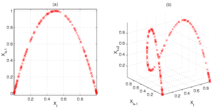
In this graph, t has been used instead of n. But it’s the same thing.
It’s the simplest possible equation with a negative feedback loop. What’s that? Let me explain. The bigger the population gets over Xₙ (this year) the smaller it will be on Xₙ₊₁ (the following year).
Still not clear? Alright, let’s understand this with examples.
Let r be 3.4, and the starting population Xₙ be 0.3 (30% of the maximum population). Upon calculating, we get 0.816. Okay, so the population increased from 0.3 to 0.816 in the first year. That’s a huge increment. But then if we take 0.816 as the population of this year (Xₙ), next year the population will be 0.510. Again, the year after that it will be 0.849.
But wait, there’s a catch here. After some years, the population keeps oscillating between 0.451 and 0.842 approximately. It doesn’t really change beyond that.
But wait, there’s even more. A population remains almost constant when the growth rate is 2 or near to 2. Because two children just replace their parents, so, after a certain time, the population becomes almost constant. Let’s try this out.
Suppose Xₙ is 0.35 (35% of the maximum population) and r is 2.34. So, Xₙ₊₁ will be 0.532. The year after that it will be 0.582, followed by 0.569 the year after that. After a year, the population will stabilize on 0.57. It will not increase or decrease much and will almost be fixed at 0.57, i.e, 57% of the maximum possible population. The population reaches an equilibrium.
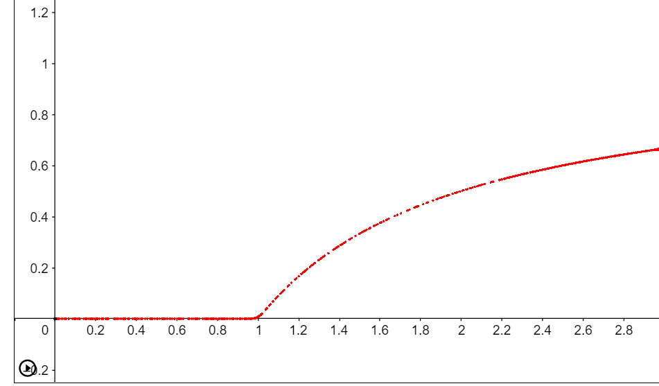
Now, even if we change the initial population, it will still reach the equilibrium sooner or later. The equilibrium number only depends on the value of r. If r is lower, then the equilibrium population gets lower and if it is lesser than 1, then the population gets to 0 sooner or later.
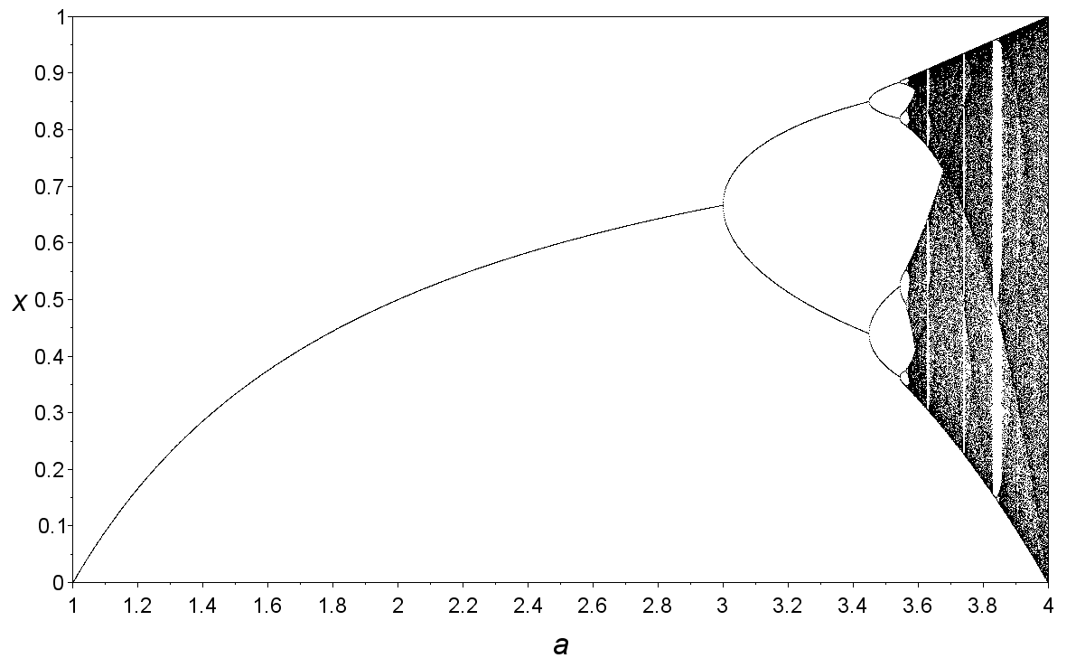
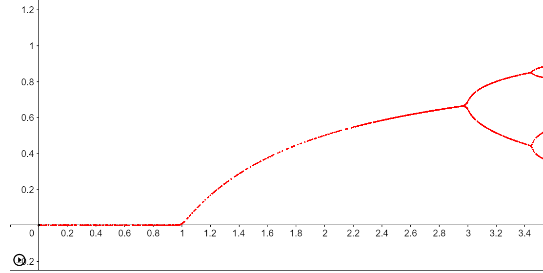
Now, let’s make another graph with r (growth rate) on x axis and the equilibrium population on y axis. At first, when r is lesser than 1, the equilibrium population remains 0. But upon r crossing 1, the equilibrium population keeps increasing.
But something interesting happens when r passes 3 and maybe you can guess it too. Remember when we kept r=3.4. The equilibrium population kept oscillating between 0.84 and 0.51. After that, if never settles down to a constant value and it oscillates back and forth between two values instead. One year the population is higher and the next year it is lower and then it is higher again in the following year.
As time passes, the equilibrium population splits into 4 values. The population repeats after a 4-year cycle.
Since the length of the cycle has doubled, it is called period-doubling bifurcations. as r increases, it leads to cycles of 8, 16, 32 and when r reaches about 3.57, it’s complete chaos. Then the population never settles down at all.
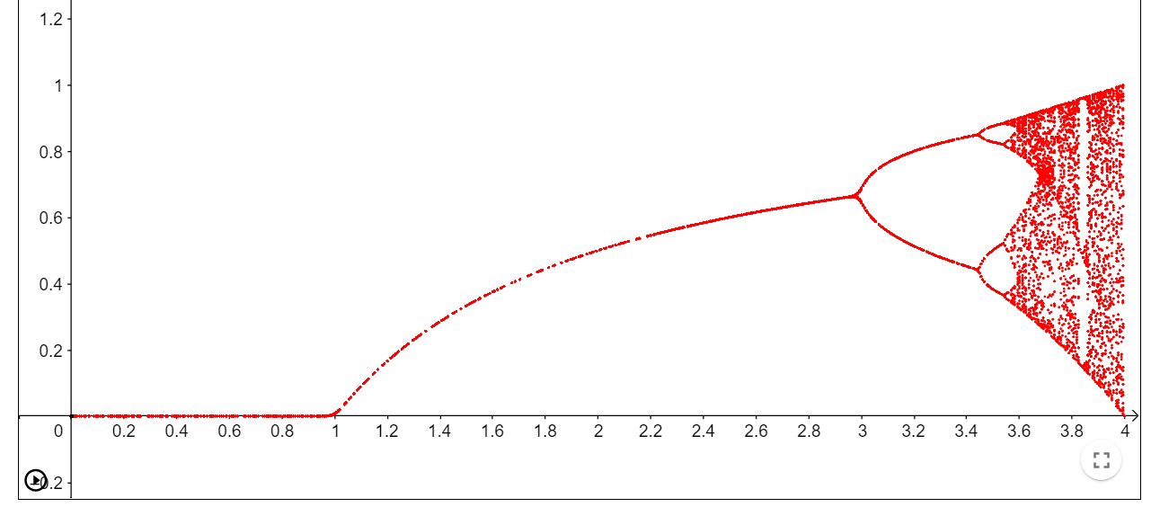
The population just becomes random. It is so random that this was one of the primary methods of generating random numbers in computers. This way, a deterministic machine gave an unpredictable answer. Although there is no repeating, if you know the initial values, you can calculate the given values. So, it’s actually pseudo-random.
Wait, look at the graph at around r= 3.83 approximately. There is a small portion where the order returned. The population repeated after 3 years. The cycle was of 3 years. As r grows more and more, the cycle splits into 6, 12, 24 and then chaos again.
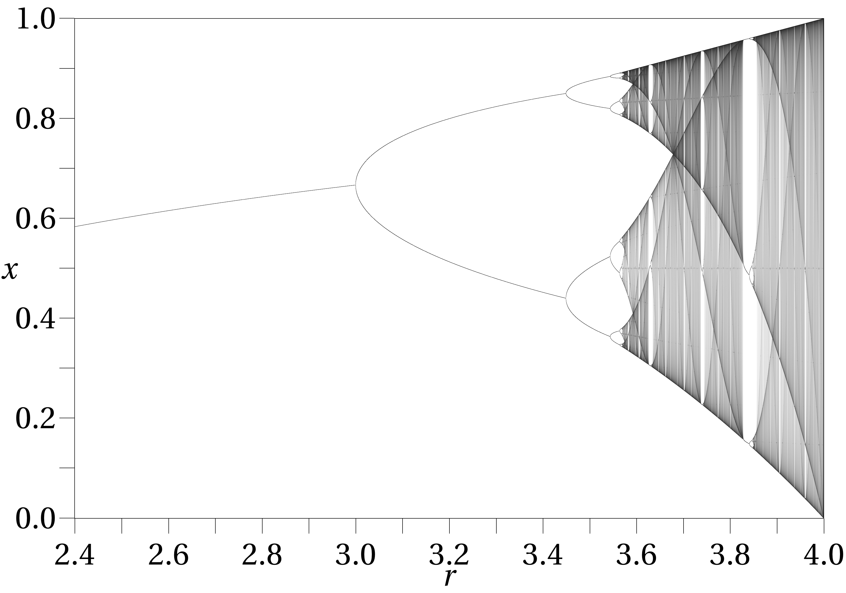
You might be thinking, it looks like a fractal. Well, it is. The large scale features are repeated on a smaller scale.
Probably the most famous fractal is the Mandelbrot set.

Well, there’s a surprise for you. The bifurcation diagram is actually a part of the Mandelbrot set.

Cool, right?
What the heck is a Mandelbrot set?
It is based on the simple equation, Zₙ₊₁ = Zₙ² + C. So, pick a number C, any number in the complex plane, then start calculating Zₙ₊₁ starting from Zₙ = 0. Now, iterate this equation again and again and again and again and… You get my point.
Now, if the number blows up to infinity, then that number (what we assumed as C) is not a part of the Mandelbrot set. But, if that number remains finite after unlimited iterations, it is part of the Mandelbrot set.
For example, if C=3, after the first iteration, Zₙ₊₁=3. After the second iteration, Zₙ₊₁=12. After the third iteration, Zₙ₊₁=147. After unlimited iterations, Zₙ₊₁ will be infinity. So, 3 will not be a part of the Mandelbrot set.
Again, if C=-1, after the first iteration, Zₙ₊₁=-1. After the second iteration, Zₙ₊₁=0. After the third iteration, Zₙ₊₁=-1. After the fourth iteration Zₙ₊₁=0 again. The value of Zₙ₊₁ oscillates between -1, and 0. So, -1 is a part of the Mandelbrot set.
The picture of the Mandelbrot set just shows the boundary between the numbers that cause the iterated equation to blow up and those that cause it to blow up. What the Mandelbrot set doesn’t show is how these equations remain finite. So, we iterated the equation thousands of times and plotted on the z axis the iteration actually takes. So, the side view of the Mandelbrot set is actually the bifurcation diagram.
All of the numbers in the main cardioid end up stabilizing on a single constant and the numbers in the main bulb oscillate between two values. In the smaller bulb, they oscillate between four values and so on. The chaotic part of the bifurcation diagram happens on the needle of the Mandelbrot set. Now, look at the medallion in the middle of the needle part. That part is when the bifurcation plot stabilizes for a small window.
How beautiful and mind-boggling this is!
Now, I claimed that this equation determines the population of a species. Is this true? Well, yes. Especially in laboratory conditions. Not only this, the equation applies to a huge variety of different areas of science and often those areas of science are unrelated to each other.
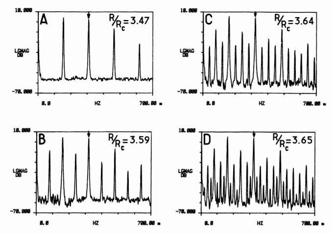
Albert J. Libchaber’s work on fluid dynamics first confirmed this equation. His experiment included a small rectangular box with mercury inside. Then he used a small temperature gradient to induce convection, just two counter-rotating cylinders inside his box. He published his findings in a paper named ‘Period doubling cascade in mercury, a quantitative measurement’. The findings were astonishing.
An article of Publicism states,
“Libchaber used a simple pen plotter to record the temperature, as measured by a probe embedded in the top surface. In the equilibrium motion after the first bifurcation, the temperature at any one point remains steady, more or less, and the pen records a straight line. With more heating, more instability sets in. A kink develops in each roll, and the kink moves steadily back and forth. This wobble shows up as a changing temperature, up and down between two values. The pen now draws a wavy line across the paper.”
Libchaber measured the temperature of the fluid inside with a probe on the top of the box. He saw a periodic spike in the temperature. It’s similar to when the logistic equation converges to a single value. But then, as the temperature increases, a wobble can be seen on those rolling cylinders at half the original frequency. The spikes in temperature also went back and forth between two different heights. He kept increasing the temperature and he saw period-doubling again and again.
Not only this, period-doubling could be seen in many other experiments, like the response of our and Salamander’s eyes to flickering lights. Also, a lot of researchers have found our period doubling in a dripping faucet. For example, at first, you see only one drop at a time. Then two drops at a time. Then four… You achieve chaotic behaviour from a dripping faucet just by adjusting the knob.
Now if the bifurcation diagram already looks spooky to you, hold on, we got more. Physicist Mitchen Feigenbaum divided the width of each bifurcations section by the next one. That ratio closed into a number. It’s 4.669. That’s like, 4.6Nice.
Jokes apart, the number 4.669 is now called the Feigenbaum constant. The bifurcations come faster to the right but the ratio is always approaching to this fixed value of 4.669.
Now, 4.669 is thought to be a fundamental constant because it doesn’t relate to any other existing physical constant in the universe. But wait, not only the equation I wrote at the beginning of this article obey this. Any equation that has a single hump (for example, Xₙ₊₁ = sinx), if you iterate it again and again, you will be bifurcations. Even the ratio of when these bifurcations occur will be the same, 4.669.
The bifurcation diagram and the Feigenbaum constant is thought to be universal. Because it appears in so many places in mathematics and physics. This universality is truly amazing.
So, yeah. That’s the equation that rules the universe. Well, let me correct myself a bit. It’s not just an equation, it’s the bifurcation diagram and the Feigenbaum constant. So, that’s an equation that has a single bump behaves the same way.
I hope more researches are made in this field and the Feigenbaum constant is checked in more phenomenons in nature. Only that way we will be able to unravel its true power.
This article is heavily inspired by an article on Publicism, a video by Veritasium, and Libchaber’s paper, named ‘Period doubling cascade in mercury, a quantitative measurement’.

Written by
Developer, designer, writer, data analyst, AI specialist. https://www.patreon.com/SamratDuttaOfficial https://www.instagram.com/samratduttaofficial

Cryorus
Great exposition, this is also why the #Asynsis principle is an elegant new green, design law of nature and culture.
Here's my QED, first published in AD Magazine in 1994, and as shared on TED conferences, plus how we can apply it via #MetaLoop…...
5
Well done. thanks for the examples. Only one criticism: it appears that your essay had been nidely edited until this paragraph when the wording began to deteriorate: "Now if the bifurcation diagram already looks spooky to you, hold on, we got more…...
5
My article with code examples.
3
I think this article misses some really important aspects, because although the equation shows the process from determinism to chaos it doesn't rule the world. Rule is the operative word.
This is because it's not the only thing going. The presence of…...